---
title: "NFL EndZone Pipeline Weekly Report Playbook"
description: "Draft walkthrough of the nflendzonePipeline weekly-report vignette and the six core outputs it generates each run."
author: Tyler Pollard
date: 2026-02-15
date-modified: 2026-02-15
draft: false
categories:
- nflendzone
- nflverse
- pipeline
- etl
- data-engineering
# image: false
# image: index_files/figure-html/team-strength-plot-2.png
repo-url: "https://github.com/TylerPollard410/nflendzonePipeline"
---
[View repository source {{< bi github >}}]({{< meta repo-url >}}){.btn .btn-warning target="_blank"}
This draft post is based on `vignettes/weekly-report.qmd` in `nflendzonePipeline`. The goal is to keep one practical readout of what changes each week, why it changes, and what should be checked in model/app outputs next. While the rendered weekly report as seen on the [repository]({{< meta repo-url >}}) will continue to evolve, this post will serve as a stable reference for the core workflow and outputs that are generated each week.
## Workflow At A Glance
```{mermaid}
flowchart LR
  A[nflverse raw data] --> B[nflendzonePipeline ETL + features]
  B --> C[nflendzoneData release tags]
  C --> D[weekly-report.qmd]
  D --> E[nflendzoneModel checks]
  D --> F[nflendzoneApp probability views]
```
## Core Steps Used In The Vignette
1. Load schedules, teams, and game history from `nflreadr`.
2. Pull latest `*_filter` and `*_predict` assets from `nflendzoneData` release tags.
3. Standardize variable names (`filtered_` and `predicted_` prefixes).
4. Render team strength, HFA, spread, win probability, score distribution, and betting-edge visuals.
## Weekly Checklist I Use
- Confirm timestamp files and week/season labels match expected run window.
- Look for team-level movement with uncertainty widening, not just mean shifts.
- Flag sudden market-edge changes and trace them back to latent state movement.
- Hand off findings to model refresh and app QA.
{{< include ../../../_footer.qmd >}}
# Weekly Report
This report provides weekly updates on NFL team strength estimates, home field advantage, and game predictions using Bayesian state-space models.
```{r}
#| label: libraries
#| code-fold: true
#| code-summary: "Show the R code - libraries"
# Core data manipulation
library(dplyr)
library(purrr)
library(stringr)
# library(readr)      # optional: file I/O helpers (not used here)
# library(lubridate)  # optional: date/time tools (not used here)

# Plotting and colors
library(ggplot2)
library(ggdist)
library(colorspace)
library(grid) # for unit()
# library(bayesplot)   # optional: Bayesian plotting helpers (not used here)
# library(patchwork)   # optional: plot composition (not used here)

# Bayesian random variables and helpers (E, Pr, rvar)
library(posterior)
# library(distributional)  # optional: distributions/rvars (not called directly)
# library(tidybayes)       # optional: tidy extraction of Bayesian fits (not used here)

# NFL packages (keep these five at the end)
library(nflreadr)
library(nflplotR)
# library(nflendzone)   # old app repo
# library(nflendzoneModel) # modeling repo; listing for reference
library(nflendzonePipeline)

# Theming
library(bslib)
library(brand.yml)
library(quarto)

# theme_set(theme_ggdist())
```
```{r}
#| label: theme-setup
project_root <- find_project_root(path = ".")
light_brand_yml <- read_brand_yml(file.path(
  project_root,
  "_extensions/TylerPollard410/my-brand/brand-light.yml"
))
dark_brand_yml <- read_brand_yml(file.path(
  project_root,
  "_extensions/TylerPollard410/my-brand/brand-dark.yml"
))

base_text_size <- 17

# theme from brands
theme_brand_light <- brand.yml::theme_brand_ggplot2(
  brand = light_brand_yml,
  # background = NULL,
  # foreground = NULL,
  # accent = NULL,
  # ...,
  base_size = base_text_size,
  title_size = base_text_size * 1.2
  # title_color = NULL,
  # line_color = NULL,
  # rect_fill = NULL,
  # text_color = NULL,
  # plot_background_fill = NULL,
  # panel_background_fill = NULL,
  # panel_grid_major_color = NULL,
  # panel_grid_minor_color = NULL,
  # axis_text_color = NULL,
  # plot_caption_color = NULL
)

theme_brand_dark <- brand.yml::theme_brand_ggplot2(
  brand = dark_brand_yml,
  base_size = base_text_size,
  title_size = base_text_size * 1.2
)
```
## Data Setup
Load game data and team information from all available seasons.
```{r}
#| label: globals
#| code-fold: true
#| code-summary: "Show the R code - globals"
all_seasons <- 2002:nflreadr::most_recent_season()
teams_data <- nflreadr::load_teams(current = TRUE)
game_data <- nflendzonePipeline::load_game_data(seasons = all_seasons)
game_data_long <- nflendzonePipeline::load_game_data_long(game_df = game_data)
season_weeks_df <- game_data |>
  dplyr::distinct(season, week, week_seq)

base_repo_url <-
  "https://github.com/TylerPollard410/nflendzoneData/releases/download/"

# Create named vector of team colors (lightened for visibility)
team_colors <- setNames(teams_data$team_color, teams_data$team_abbr)
team_colors_light <- colorspace::lighten(team_colors, amount = 0.25)
team_colors_dark <- colorspace::lighten(team_colors, amount = 0.95)
```
## Load Model Estimates
Extract the latest filtered and predicted estimates from the data repository.
```{r}
#| label: load-estimates-data-function
#| code-fold: true
#| code-summary: "Show the R code - load-estimates-data-function"
# Function to load timestamps and estimates for a given set of tags
load_estimates_data <- function(tags, base_url) {
  # Load timestamps
  timestamps <- purrr::map(
    tags,
    ~ {
      timestamp_url <-
        paste0(base_url, .x, "/", .x, "_timestamp.json")
      jsonlite::fromJSON(timestamp_url)
    }
  ) |>
    purrr::set_names(tags)

  # Load estimates using season and week from timestamp data
  estimates <- purrr::imap(
    timestamps,
    ~ {
      # Extract season and week from timestamp
      season <- .x$season
      week <- .x$week
      week_idx <- .x$week_idx

      # Build URL with season and week in filename
      data_url <-
        paste0(base_url, .y, "/", .y, "_", season, "_", week, ".rds")
      data <- nflreadr::rds_from_url(data_url)

      # Attach timestamp as attributes
      attr(data, "season") <- season
      attr(data, "week") <- week
      attr(data, "week_idx") <- week_idx

      return(data)
    }
  )

  return(estimates)
}
```
```{r}
#| label: extract-estimates
#| code-fold: true
#| code-summary: "Show the R code - extract-estimates"
# Define both sets of tags
filter_tags <- c(
  "team_strength_filter",
  "league_hfa_filter",
  "result_filter"
)

predict_tags <- c(
  "team_strength_predict",
  "league_hfa_predict",
  "result_predict"
)

# Load filter data
filter_data <- load_estimates_data(filter_tags, base_repo_url)

# Load predict data
predict_data <- load_estimates_data(predict_tags, base_repo_url)
```
```{r}
#| label: extract-estimates-example
#| cahce: true
#| echo: false
#| warning: false
last_reg_week <- game_data |>
filter(season == max(season), season_type == "REG") |>
last() |>
select(season, week, week_seq) |>
left_join(season_weeks_df) |>
rename(week_idx = week_seq)
first_post_week <- last_reg_week |>
mutate(
week = week + 1,
week_idx = week_idx + 1
) |>
as.list()
last_reg_week <- last_reg_week |>
as.list()
# Define both sets of tags
filter_tags <- c(
"team_strength_filter",
"league_hfa_filter",
"result_filter"
)
filter_tags <- rep(list(last_reg_week), length(filter_tags)) |>
setNames(filter_tags)
predict_tags <- c(
"team_strength_predict",
"league_hfa_predict",
"result_predict"
)
predict_tags <- rep(list(first_post_week), length(predict_tags)) |>
setNames(predict_tags)
estimates_func <- function(timestamps, base_url) {
purrr::imap(
timestamps,
~ {
# Extract season and week from timestamp
season <- .x$season
week <- .x$week
week_idx <- .x$week_idx
# Build URL with season and week in filename
data_url <-
paste0(base_url, .y, "/", .y, "_", season, "_", week, ".rds")
data <- nflreadr::rds_from_url(data_url)
# Attach timestamp as attributes
attr(data, "season") <- season
attr(data, "week") <- week
attr(data, "week_idx") <- week_idx
return(data)
}
)
}
# Load filter data
filter_data <- estimates_func(filter_tags, base_repo_url)
# Load predict data
predict_data <- estimates_func(predict_tags, base_repo_url)
```
```{r}
#| label: clean-data
#| cahce: true
#| code-fold: true
#| code-summary: "Show the R code - clean-data"
# Clean up filter data
filter_data <- filter_data |>
  purrr::map(
    \(x) {
      x |>
        dplyr::rename_with(
          ~ stringr::str_remove(.x, "^filtered_")
        ) |>
        mutate(type = "filter")
    }
  )


# Clean up predict data
predict_data <- predict_data |>
  purrr::map(
    \(x) {
      x |>
        dplyr::rename_with(
          ~ stringr::str_remove(.x, "^predicted_")
        ) |>
        mutate(type = "predict")
    }
  )
```
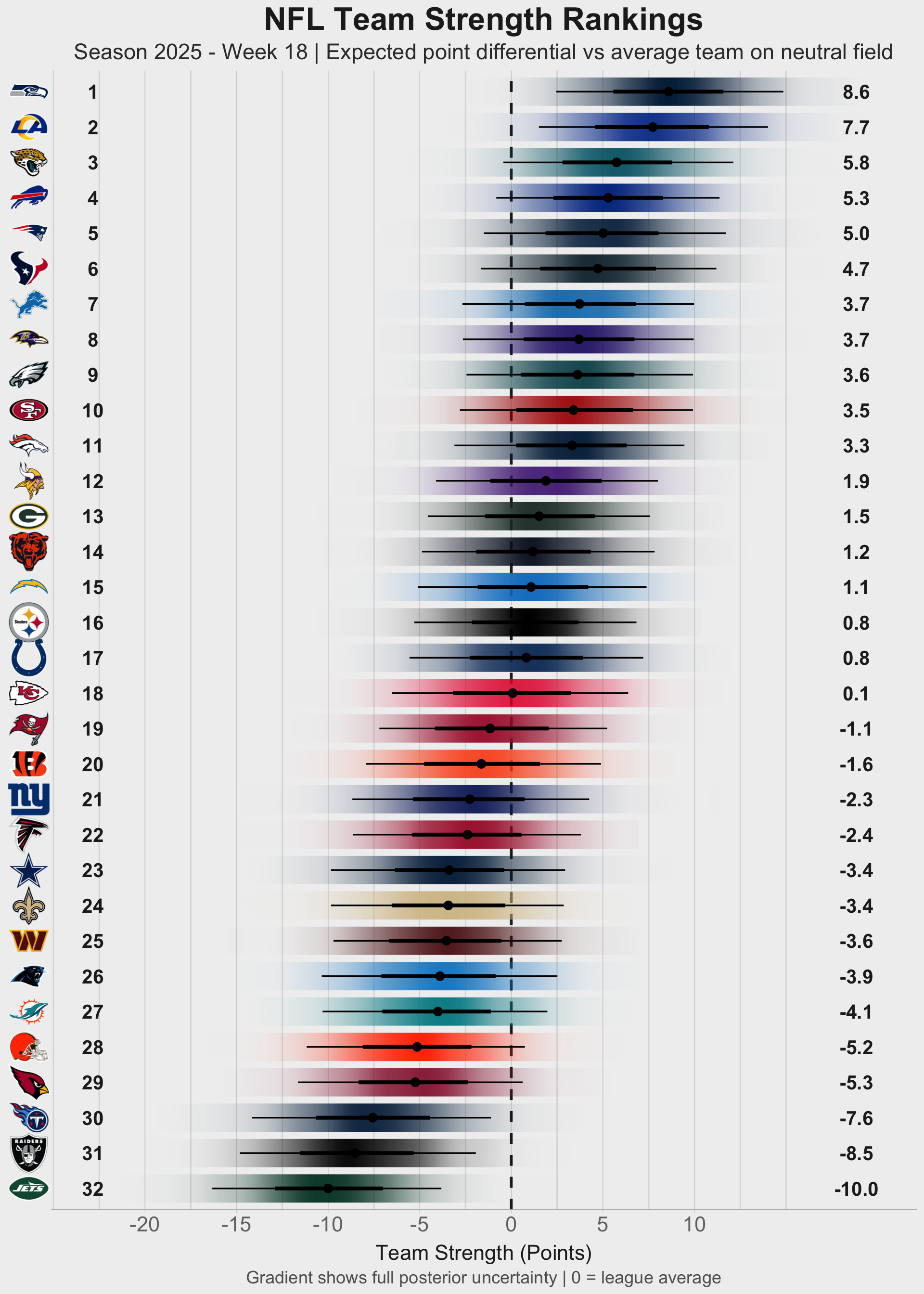
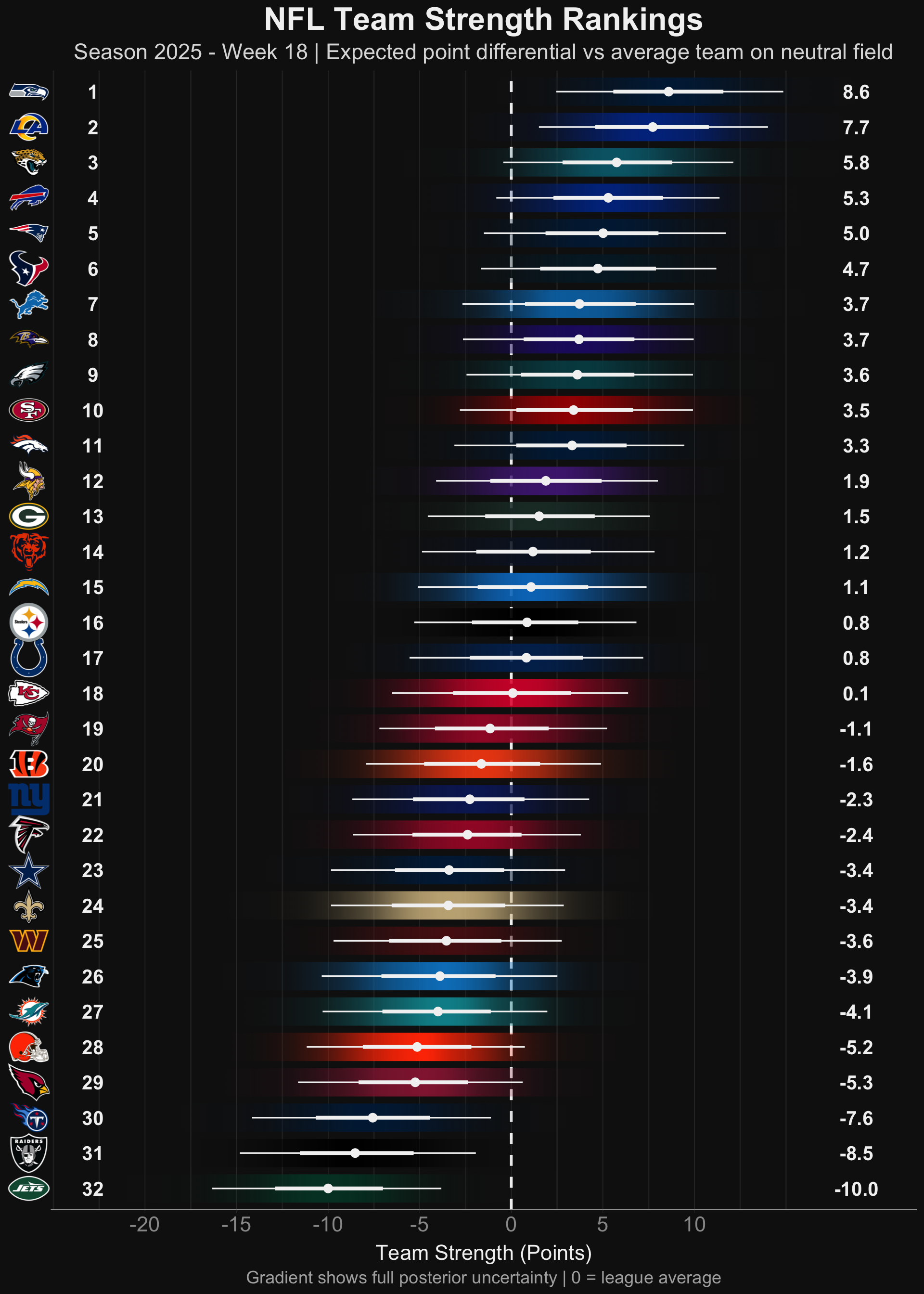
## Team Strength Rankings
Current team strength estimates ranked from strongest to weakest. Values
represent the expected point differential against an average team on a neutral
field. The gradient intervals show the full posterior distribution.
```{r}
#| label: team-strength-plot
#| renderings: [dark, light]
#| code-fold: true
#| code-summary: "Show the R code - team-strength-plot"
#| fig-align: center
#| fig-width: 10
#| fig-height: 14
# Filter for the latest week
team_strength_filter_df <- filter_data |>
  pluck("team_strength_filter") |>
  left_join(teams_data, by = c("team" = "team_abbr")) |>
  arrange(desc(E(team_strength))) |>
  mutate(rank = row_number())

min_strength <- quantile(
  team_strength_filter_df$team_strength,
  probs = 0.025
) |>
  min()
max_strength <- quantile(
  team_strength_filter_df$team_strength,
  probs = 0.975
) |>
  max()
team_strength_filter_plot <- team_strength_filter_df |>
  ggplot(aes(y = reorder(team, team_strength))) +
  # Zero reference line (average team)
  geom_vline(
    xintercept = 0,
    linetype = "dashed",
    #color = "gray30",
    linewidth = 1
  ) +
  # Gradient interval showing uncertainty - lightened colors for better visibility
  stat_gradientinterval(
    aes(xdist = team_strength, fill = team),
    scale = 0.8,
    show.legend = FALSE,
    outline_bars = TRUE
  ) +
  scale_fill_nfl() +
  # scale_fill_manual(values = team_colors_light) +
  # Team logos
  # geom_nfl_logos(
  #   aes(x = (min_strength - 4), team_abbr = team),
  #   width = 0.045
  # ) +
  # Rank numbers
  geom_text(
    aes(x = (min_strength - 6.5), label = rank),
    size = base_text_size * 0.9,
    size.unit = "pt",
    fontface = "bold"
    #color = "gray10"
  ) +
  # Expected value labels - positioned to the right, outside the gradient
  geom_label(
    aes(x = (max_strength + 4), label = sprintf("%.1f", E(team_strength))),
    size = base_text_size * 0.9,
    size.unit = "pt",
    border.color = NA,
    fontface = "bold",
    fill = NA,
    alpha = 0.9,
    label.padding = unit(0.2, "lines")
    #position = position_jitter(width = 0, height = 0.15, seed = 42)
  ) +
  scale_x_continuous(
    breaks = seq((min_strength %/% 5) * 5, (max_strength %/% 5) * 5, 5),
    limits = c(round(min_strength - 7), round(max_strength + 5))
  ) +
  labs(
    title = "NFL Team Strength Rankings",
    subtitle = paste(
      "Season",
      attr(filter_data$team_strength_filter, "season"),
      "- Week",
      attr(filter_data$team_strength_filter, "week"),
      "| Expected point differential vs average team on neutral field"
    ),
    x = "Team Strength (Points)",
    y = NULL,
    caption = "Gradient shows full posterior uncertainty | 0 = league average"
  ) +
  theme_ggdist() +
  #theme_brand_light +
  theme(
    plot.title = element_text(face = "bold", hjust = 0.5),
    plot.subtitle = element_text(size = rel(1), hjust = 0.5),
    plot.caption = element_text(size = rel(1.5), hjust = 0.5), #color = "gray40"
    axis.text.x = element_text(size = rel(1.2)),
    axis.text.y = element_nfl_logo(size = rel(1.2)),
    axis.ticks.y = element_blank(),
    axis.line.y = element_blank(),
    panel.grid.major.y = element_blank(),
    panel.grid.major.x = element_line(linewidth = 0.3) #color = "gray90",
  )

# Create copies to safely modify specific layers without affecting the original
p_dark <- team_strength_filter_plot
p_light <- team_strength_filter_plot

# Target stat_gradientinterval (Layer 2) specifically to set the ink color
# layer 1 is geom_vline, layer 2 is stat_gradientinterval
p_dark$layers[[2]]$aes_params$colour <- theme_brand_dark$geom$ink
p_dark +
  theme_brand_dark

p_light$layers[[2]]$aes_params$colour <- "black"
p_light +
  theme_brand_light
```
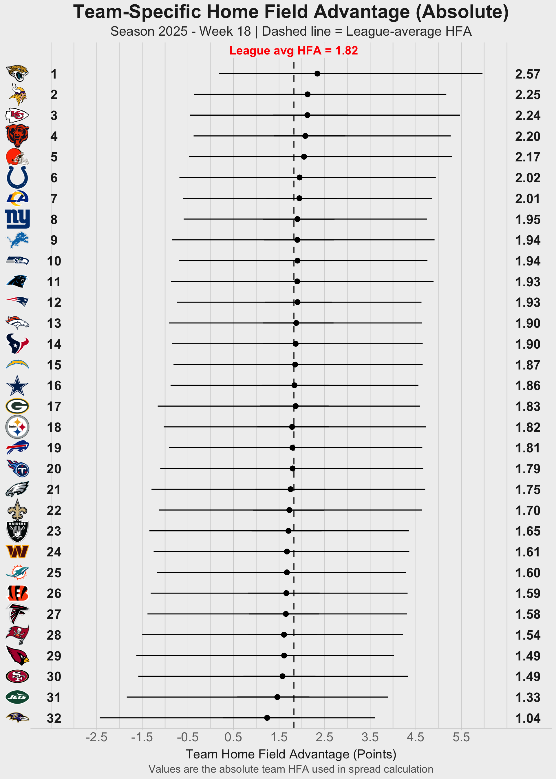
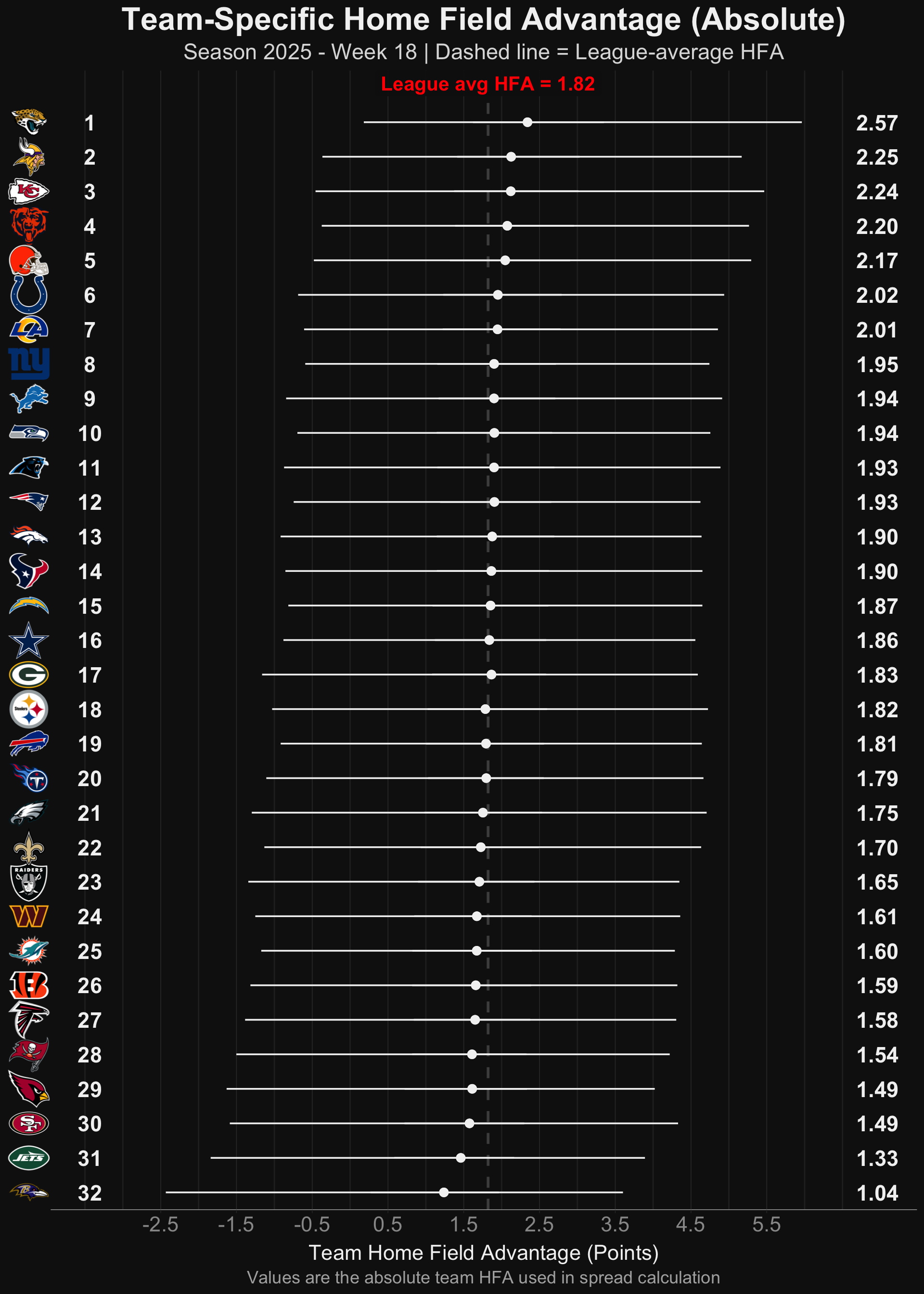
## Home Field Advantage Comparison
Team-specific home field advantages compared to league average. Values are
typically small (within ±2 points) showing modest variation around the league norm.
```{r}
#| label: hfa-comparison-plot
#| renderings: [dark, light]
#| code-fold: true
#| code-summary: "Show the R code - hfa-comparison-plot"
#| fig-align: center
#| fig-width: 10
#| fig-height: 14
# Extract league HFA and compute league average (expected value)
league_hfa_filter <- filter_data |> pluck("league_hfa_filter")
league_hfa_mean <- E(league_hfa_filter$league_hfa)

# Team-level HFA data (contains team_hfa as an rvar)
team_hfa_filter <- filter_data |> pluck("team_strength_filter")

hfa_abs_plot_df <- team_hfa_filter |>
  left_join(teams_data, by = c("team" = "team_abbr")) |>
  arrange(desc(E(team_hfa))) |>
  mutate(rank = row_number())

min_hfa <- quantile(
  hfa_abs_plot_df$team_hfa,
  probs = 0.025
) |>
  min()
max_hfa <- quantile(
  hfa_abs_plot_df$team_hfa,
  probs = 0.975
) |>
  max()

hfa_abs_plot <- hfa_abs_plot_df |>
  ggplot(aes(y = reorder(team, team_hfa))) +
  # Reference: league-average HFA
  geom_vline(
    xintercept = league_hfa_mean,
    linetype = "dashed",
    color = "gray30",
    linewidth = 1
  ) +
  # Uncertainty intervals for team HFA
  stat_pointinterval(
    aes(xdist = team_hfa, fill = team),
    .width = c(0.5, 0.95),
    point_size = 2.5,
    # interval_color = "gray20",
    # color = "gray20",
    linewidth = 1.2,
    show.legend = FALSE
  ) +
  # Inline label for league average
  annotate(
    "label",
    x = league_hfa_mean,
    y = Inf,
    label = sprintf("League avg HFA = %.2f", league_hfa_mean),
    vjust = 1,
    #size = base_text_size * 0.9,
    fontface = "bold",
    text.color = "red",
    #fill = NA,
    alpha = 0.9,
    size = base_text_size * 0.9,
    size.unit = "pt",
    border.color = NA
  ) +
  #  scale_fill_manual(values = team_colors_light) +
  # Team logos
  # geom_nfl_logos(
  #   aes(x = min_hfa - 1.0, team_abbr = team),
  #   width = 0.045
  # ) +
  # Rank numbers
  geom_text(
    aes(x = min_hfa - 1.0, label = rank),
    size = base_text_size,
    size.unit = "pt",
    fontface = "bold"
  ) +
  # Expected value labels (absolute team HFA)
  geom_label(
    aes(x = max_hfa + 1.0, label = sprintf("%.2f", E(team_hfa))),
    size = base_text_size,
    size.unit = "pt",
    border.color = NA,
    fontface = "bold",
    fill = NA,
    alpha = 0.9,
    label.padding = unit(0.2, "lines")
  ) +
  scale_y_discrete(
    expand = expansion(add = c(0.5, 1.5))
  ) +
  scale_x_continuous(
    breaks = seq((min_hfa %/% 0.5) * 0.5, (max_hfa %/% 0.5) * 0.5, 1)
    #limits = c(round(min_hfa) - 2, round(max_hfa) + 2),
    #limits = c(round(min_hfa), round(max_hfa))
  ) +
  labs(
    title = "Team-Specific Home Field Advantage (Absolute)",
    subtitle = paste(
      "Season",
      attr(filter_data$team_strength_filter, "season"),
      "- Week",
      attr(filter_data$team_strength_filter, "week"),
      "| Dashed line = League-average HFA"
    ),
    x = "Team Home Field Advantage (Points)",
    y = NULL,
    caption = "Values are the absolute team HFA used in spread calculation"
  ) +
  theme_ggdist() +
  theme(
    plot.title = element_text(face = "bold", hjust = 0.5),
    plot.subtitle = element_text(size = rel(1), hjust = 0.5),
    plot.caption = element_text(size = rel(1.5), hjust = 0.5), #color = "gray40"
    axis.text.x = element_text(size = rel(1.2)),
    axis.text.y = element_nfl_logo(size = rel(1.2)),
    # axis.text.y = element_text(size = rel(1.2)),
    axis.ticks.y = element_blank(),
    axis.line.y = element_blank(),
    panel.grid.major.y = element_blank(),
    panel.grid.major.x = element_line(linewidth = 0.3) #color = "gray90",
  )

# Create copies to safely modify specific layers without affecting the original
p_dark <- hfa_abs_plot
p_light <- hfa_abs_plot

# Target avg label to match bg fill and stat_gradientinterval (Layer 2) specifically to set the ink color
p_dark$layers[[2]]$aes_params$colour <- theme_brand_dark$geom$ink
#p_dark$layers[[3]]$aes_params$colour <- theme_brand_dark$panel.background$fill
p_dark +
  theme_brand_dark

p_light$layers[[2]]$aes_params$colour <- "black"
#p_light$layers[[2]]$aes_params$colour <- theme_brand_light$panel.background$fill
p_light +
  theme_brand_light
```
## Weekly Game Predictions
Predicted outcomes for upcoming games with full uncertainty quantification.
```{r}
#| label: game-prediction
#| code-fold: true
#| code-summary: "Show the R code - game-prediction"
result_predict <- predict_data |>
  pluck("result_predict")
# mutate(
#   y2 = rvar_rng(rnorm, n = n(), mean = mu, sd = sigma, ndraws = 10000),
#   y3 = mu + rvar_rng(rnorm, n = n(), mean = 0, sd = sigma),
#   y4 = mu + rvar_rng(rnorm, n = 1, mean = 0, sd = 1) * sigma,
#   .after = y
# )

pred_df <- inner_join(
  result_predict,
  game_data
) |>
  mutate(
    home_mu_cover_prob = Pr(mu > spread_line),
    home_y_cover_prob = Pr(y > spread_line),
    away_mu_cover_prob = Pr(mu < spread_line),
    away_y_cover_prob = Pr(y < spread_line),
    mu_cover_prob = pmax(home_mu_cover_prob, away_mu_cover_prob),
    y_cover_prob = pmax(home_y_cover_prob, away_y_cover_prob),
    mu_cover_team = case_when(
      home_mu_cover_prob > away_mu_cover_prob ~ home_team,
      home_mu_cover_prob < away_mu_cover_prob ~ away_team,
      TRUE ~ NA_character_
    ),
    y_cover_team = case_when(
      home_y_cover_prob > away_y_cover_prob ~ home_team,
      home_y_cover_prob < away_y_cover_prob ~ away_team,
      TRUE ~ NA_character_
    ),
    mu_bet_team = ifelse(mu_cover_prob > 0.55, mu_cover_team, NA_character_),
    y_bet_team = ifelse(y_cover_prob > 0.55, y_cover_team, NA_character_)
  )
```
```{r}
#| label: prep-prediction-data
#| code-fold: true
#| code-summary: "Show the R code - prep-prediction-data"
# Prepare data with better formatting
pred_plot_df <- pred_df |>
  mutate(
    matchup = paste0(away_team, " @ ", home_team),
    matchup_display = if_else(
      hfa == 1,
      paste0(away_team, " @ ", home_team),
      paste0(away_team, " vs ", home_team, " (N)")
    )
  ) |>
  #rowwise() |>
  # mutate(
  #   spread_line_y_prob = density(y, at = spread_line)
  # ) |>
  #ungroup() |>
  arrange(game_idx)
```
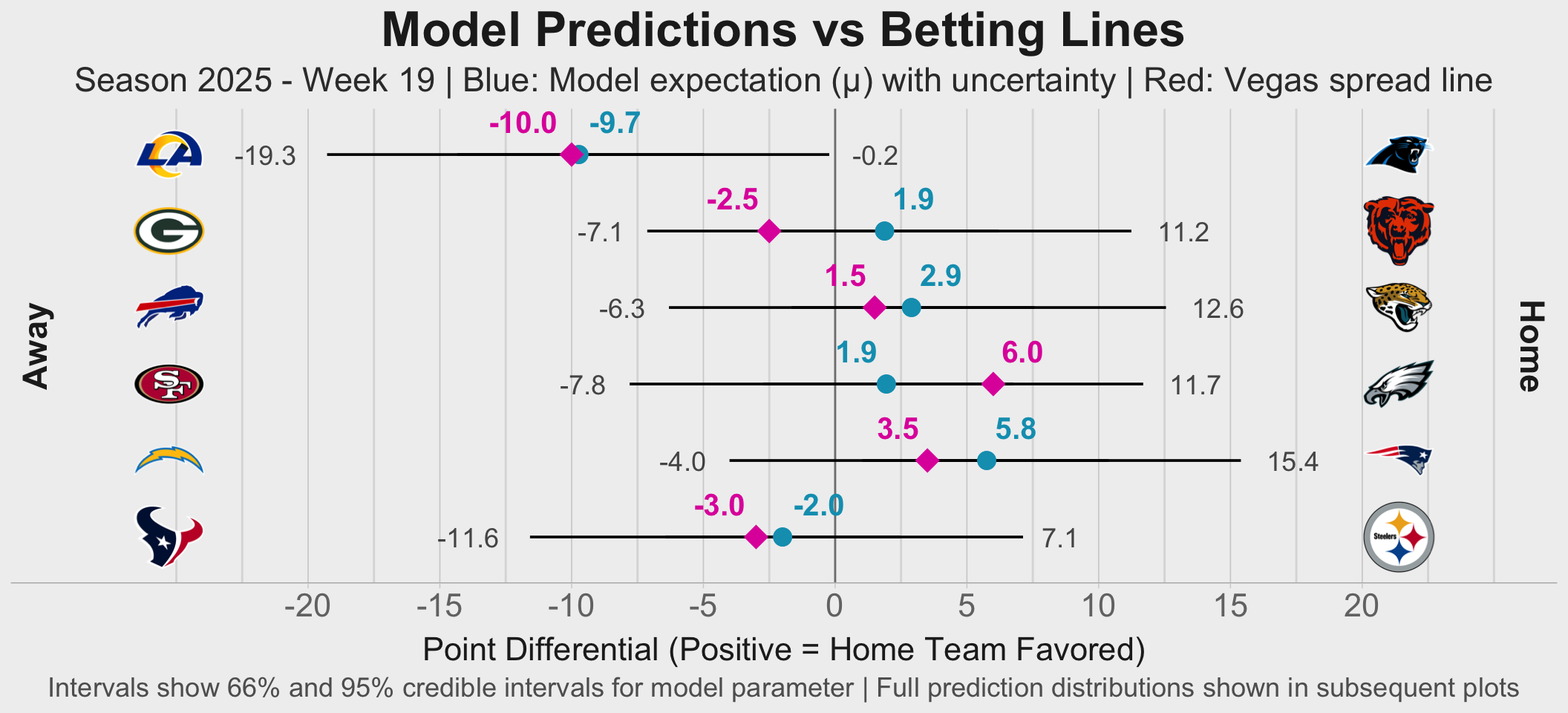
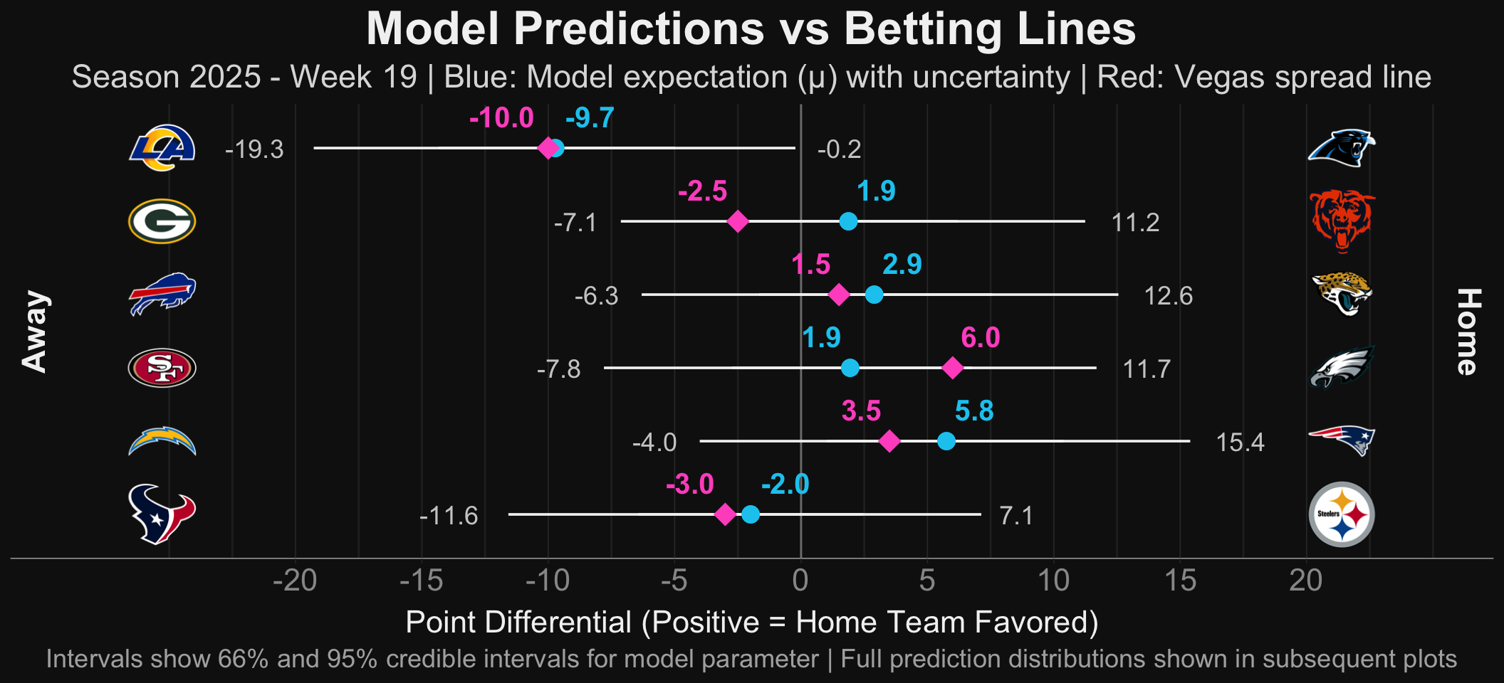
### Expected Point Spreads vs Betting Lines
How our model's expected spread compares to Vegas betting lines. Points show the
expected differential with uncertainty intervals.
```{r}
#| label: spread-comparison-plot
#| renderings: [dark, light]
#| code-fold: true
#| code-summary: "Show the R code - spread-comparison-plot"
#| fig-align: center
#| fig-width: 11
# fig-height: 8

# Calculate dynamic x-axis limits based on mu distribution
min_mu_data <- quantile(
  pred_plot_df$mu,
  probs = 0.025
) |>
  min()
max_mu_data <- quantile(
  pred_plot_df$mu,
  probs = 0.975
) |>
  max()

# Calculate logo and text positions
away_logo_pos_spread <- min_mu_data - 5
home_logo_pos_spread <- max_mu_data + 5

# Calculate x-axis limits
x_min_spread <- floor((min_mu_data - 5) / 5) * 5
x_max_spread <- ceiling((max_mu_data + 5) / 5) * 5

spread_plot <- pred_plot_df |>
  rowwise() |>
  mutate(
    # Calculate interval bounds for labels (per-game)
    mu_lower_95 = median(quantile(mu, 0.025)),
    mu_upper_95 = median(quantile(mu, 0.975)),
    # Check if spread and mu are close (for label positioning)
    values_close = abs(spread_line - median(mu)) < 3
  ) |>
  ungroup() |>
  ggplot(aes(y = reorder(matchup_display, game_idx, decreasing = TRUE))) +
  # Zero reference line
  geom_vline(
    xintercept = 0,
    linetype = "solid",
    color = "gray50",
    linewidth = 0.5
  ) +
  # Expected value (mu) - model's best estimate with uncertainty
  stat_pointinterval(
    aes(xdist = mu, color = "Model", interval_color = "ink"),
    .width = c(0.66, 0.95),
    point_size = 3.5,
    linewidth = 1.3
    #color = "#013369",
    # interval_color = "black"
  ) +
  # Betting spread line - on top so visible
  geom_point(
    aes(x = spread_line, color = "Vegas"),
    #color = "#D50A0A",
    size = 5.5,
    shape = 18
  ) +
  # 95% interval bound labels
  geom_text(
    aes(
      x = mu_lower_95,
      label = sprintf("%.1f", mu_lower_95)
    ),
    vjust = 0.5,
    hjust = 1.5,
    size = base_text_size * 0.8,
    size.unit = "pt",
    #color = "#013369",
    alpha = 0.8
  ) +
  geom_text(
    aes(
      x = mu_upper_95,
      label = sprintf("%.1f", mu_upper_95)
    ),
    vjust = 0.5,
    hjust = -0.5,
    size = base_text_size * 0.8,
    size.unit = "pt",
    #color = "#013369",
    alpha = 0.8
  ) +
  # Spread line value label (horizontal positioning: lower value shifts left)
  geom_text(
    aes(
      x = spread_line,
      label = sprintf("%.1f", spread_line),
      hjust = if_else(spread_line < median(mu), 1.2, -0.2),
      color = "Vegas"
    ),
    vjust = -1,
    size = base_text_size * 0.9,
    size.unit = "pt",
    fontface = "bold"
    #color = "#D50A0A"
  ) +
  # Model mu value label (horizontal positioning: lower value shifts left)
  geom_text(
    aes(
      x = median(mu),
      label = sprintf("%.1f", median(mu)),
      hjust = if_else(median(mu) < spread_line, 1.2, -0.2),
      color = "Model"
    ),
    vjust = -1,
    size = base_text_size * 0.9,
    size.unit = "pt",
    fontface = "bold"
    #color = "#013369"
  ) +
  # Add team logos (dynamic positioning)
  geom_nfl_logos(
    aes(x = away_logo_pos_spread - 1, team_abbr = away_team),
    #aes(x = -Inf, team_abbr = away_team),
    # hjust = 0.5,
    width = 0.05
  ) +
  geom_nfl_logos(
    aes(x = home_logo_pos_spread + 1, team_abbr = home_team),
    # hjust = -0.5,
    width = 0.05
  ) +
  annotate(
    "text",
    x = -Inf,
    y = (length(unique(pred_plot_df$matchup_display)) + 1) / 2,
    label = "Away",
    vjust = 1.5,
    #hjust = -0.5,
    size = base_text_size,
    size.unit = "pt",
    angle = 90,
    fontface = "bold"
  ) +
  annotate(
    "text",
    x = Inf,
    y = (length(unique(pred_plot_df$matchup_display)) + 1) / 2,
    label = "Home",
    vjust = 1.5,
    #hjust = -0.5,
    size = base_text_size,
    size.unit = "pt",
    angle = -90,
    fontface = "bold"
  ) +
  scale_x_continuous(
    breaks = seq(
      floor(min_mu_data / 5) * 5,
      ceiling(max_mu_data / 5) * 5,
      5
    ),
    expand = expansion(add = c(6, 6))
    #limits = c(x_min_spread, x_max_spread)
  ) +
  # scale_y_discrete(
  #   "Away",
  #   labels = \(x) str_extract(x, "^[^ ]+"),
  #   sec.axis = dup_axis(
  #     name = "Home",
  #     labels =  \(y) str_extract(y, "[^ ]+$")
  #   )
  # ) +
  labs(
    title = "Model Predictions vs Betting Lines",
    subtitle = paste(
      "Season",
      attr(predict_data$result_predict, "season"),
      "- Week",
      attr(predict_data$result_predict, "week"),
      "| Blue: Model expectation (μ) with uncertainty | Red: Vegas spread line"
    ),
    x = "Point Differential (Positive = Home Team Favored)",
    y = NULL,
    caption = "Intervals show 66% and 95% credible intervals for model parameter | Full prediction distributions shown in subsequent plots"
  ) +
  theme_ggdist() +
  theme(
    plot.title = element_text(face = "bold", hjust = 0.5),
    plot.subtitle = element_text(size = rel(1), hjust = 0.5),
    plot.caption = element_text(size = rel(1.5), hjust = 0.5), #color = "gray40"
    axis.text.x = element_text(size = rel(1.2)),
    # axis.text.y = element_nfl_logo(size = rel(1.2)),
    # axis.text.y = element_text(size = rel(1.2)),
    axis.text.y = element_blank(),
    axis.ticks.y = element_blank(),
    axis.line.y = element_blank(),
    panel.grid.major.y = element_blank(),
    panel.grid.major.x = element_line(linewidth = 0.3), #color = "gray90",
    legend.position = "none"
  )

# Create copies to safely modify specific layers without affecting the original
p_dark <- spread_plot
p_light <- spread_plot

# Target avg label to match bg fill and stat_gradientinterval (Layer 2) specifically to set the ink color
# p_dark$layers$layer_slabinterval$aes_params$interval_colour <- theme_brand_dark$geom$ink
#p_dark$layers[[3]]$aes_params$colour <- theme_brand_dark$panel.background$fill
p_dark +
  scale_color_manual(
    aesthetics = "interval_colour",
    values = c(theme_brand_dark$geom$ink)
  ) +
  scale_color_manual(
    values = c(
      brand_pluck(dark_brand_yml, "color", "info"),
      brand_pluck(dark_brand_yml, "color", "danger")
    )
  ) +
  theme_brand_dark

#p_light$layers$layer_slabinterval$aes_params$interval_colour <- "black"
#p_light$layers[[2]]$aes_params$colour <- theme_brand_light$panel.background$fill
p_light +
  scale_color_manual(
    aesthetics = "interval_colour",
    values = "black"
  ) +
  scale_color_manual(
    values = c(
      darken(brand_pluck(light_brand_yml, "color", "info"), 0.2),
      darken(brand_pluck(light_brand_yml, "color", "danger"), 0.2)
    )
  ) +
  theme_brand_light
```
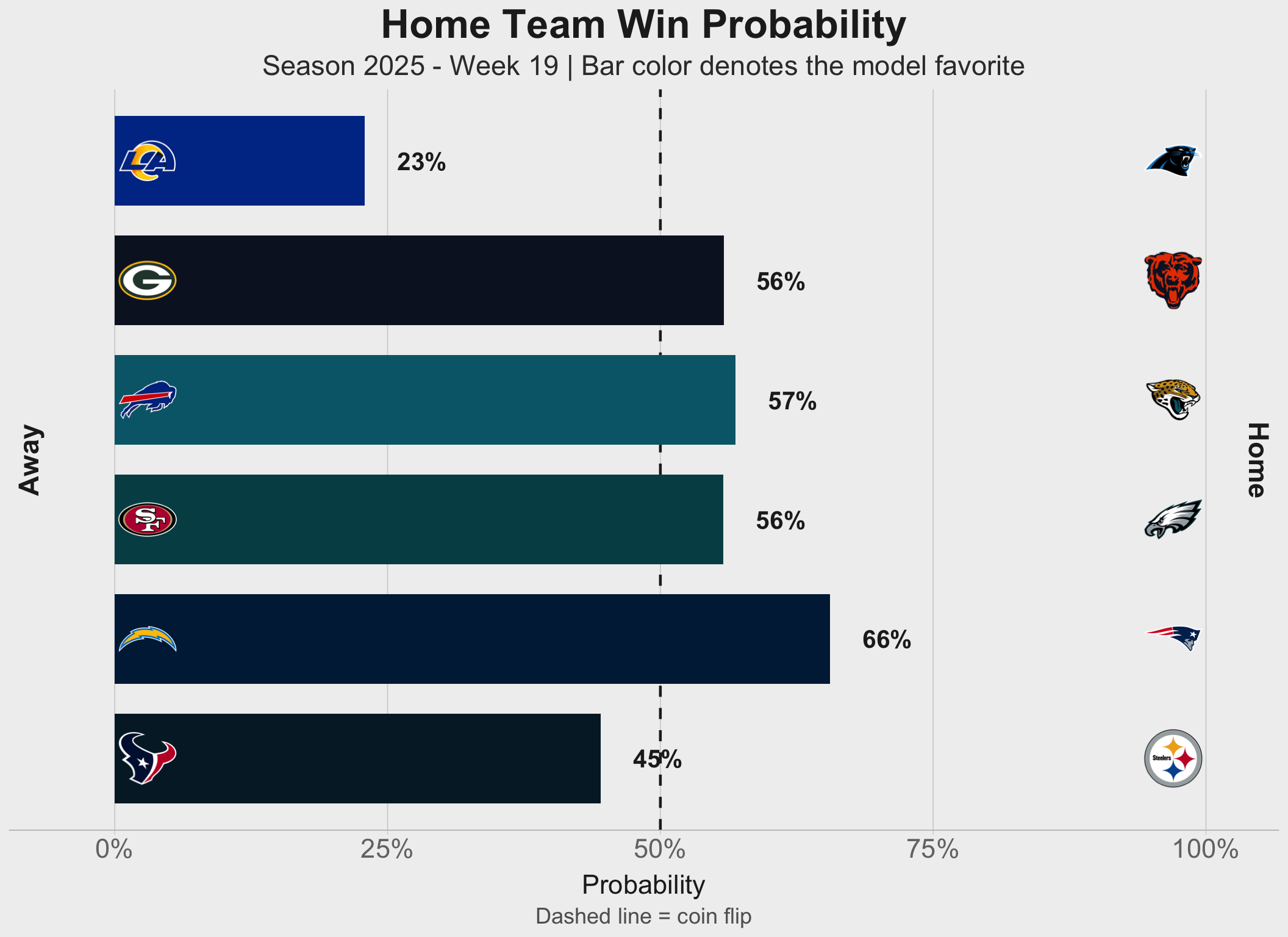
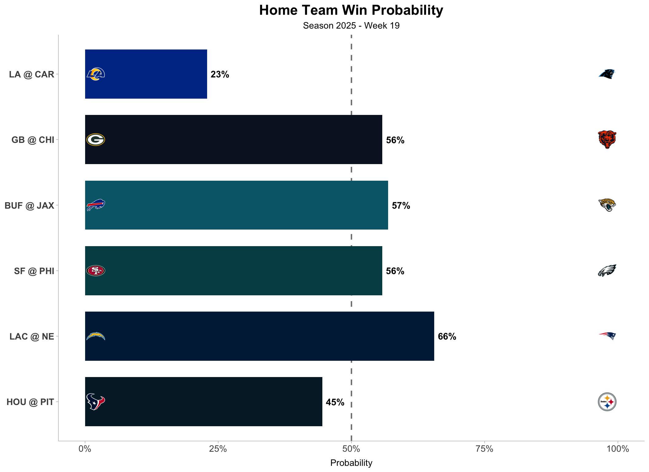
### Win Probability by Game
Probability that the home team wins each matchup.
```{r}
#| label: win-prob-plot-legacy-reference
#| eval: false
#| include: false
# Old chunk retained for reference:
# ```{r}
# #| label: win-prob-plot
# #| code-fold: true
# #| code-summary: "Show the R code - win-prob-plot"
# #| fig-align: center
# #| fig-width: 11
# #| fig-height: 8
#
# win_prob_plot <- pred_plot_df |>
# mutate(
# home_win_prob = Pr(y > 0),
# away_win_prob = 1 - home_win_prob,
# favored_team = if_else(home_win_prob > 0.5, home_team, away_team),
# favored_color = if_else(
# home_win_prob > 0.5,
# team_colors[home_team],
# team_colors[away_team]
# )
# ) |>
# ggplot(aes(y = reorder(matchup_display, game_idx, decreasing = TRUE))) +
# geom_vline(
# xintercept = 0.5,
# linetype = "dashed",
# color = "gray50",
# linewidth = 0.8
# ) +
# geom_col(
# aes(x = home_win_prob, fill = favored_team),
# width = 0.75
# ) +
# geom_text(
# aes(
# x = home_win_prob,
# label = scales::percent(home_win_prob, accuracy = 1)
# ),
# hjust = -0.2,
# size = 4,
# fontface = "bold"
# ) +
# geom_nfl_logos(
# aes(x = 0.02, team_abbr = away_team),
# width = 0.035
# ) +
# geom_nfl_logos(
# aes(x = 0.98, team_abbr = home_team),
# width = 0.035
# ) +
# scale_fill_manual(values = team_colors) +
# scale_x_continuous(
# labels = scales::percent,
# limits = c(0, 1.00),
# breaks = seq(0, 1, 0.25)
# ) +
# labs(
# title = "Home Team Win Probability",
# subtitle = paste(
# "Season",
# attr(predict_data$result_predict, "season"),
# "- Week",
# attr(predict_data$result_predict, "week")
# ),
# x = "Probability",
# y = NULL
# ) +
# theme_ggdist() +
# theme(
# plot.title = element_text(size = 17, face = "bold", hjust = 0.5),
# plot.subtitle = element_text(size = 11, hjust = 0.5),
# axis.text.y = element_text(size = 11, face = "bold"),
# axis.text.x = element_text(size = 11),
# panel.grid.major.y = element_blank(),
# panel.grid.minor.x = element_blank(),
# legend.position = "none"
# )
#
# win_prob_plot
# ```
```
```{r}
#| label: win-prob-plot
#| renderings: [dark, light]
#| code-fold: true
#| code-summary: "Show the R code - win-prob-plot"
#| fig-align: center
#| fig-width: 11
#| fig-height: 8
win_prob_plot <- pred_plot_df |>
  mutate(
    home_win_prob = Pr(y > 0),
    away_win_prob = 1 - home_win_prob,
    favored_team = if_else(home_win_prob > 0.5, home_team, away_team),
    label_x = pmin(home_win_prob + 0.03, 0.985),
    label_hjust = if_else(home_win_prob > 0.94, 1, 0)
  ) |>
  ggplot(aes(y = reorder(matchup_display, game_idx, decreasing = TRUE))) +
  geom_vline(
    xintercept = 0.5,
    linetype = "dashed",
    linewidth = 0.8
  ) +
  geom_col(
    aes(x = home_win_prob, fill = favored_team),
    width = 0.75
  ) +
  geom_text(
    aes(
      x = label_x,
      label = scales::percent(home_win_prob, accuracy = 1),
      hjust = label_hjust
    ),
    size = base_text_size * 0.9,
    size.unit = "pt",
    fontface = "bold"
  ) +
  geom_nfl_logos(
    aes(x = 0.03, team_abbr = away_team),
    width = 0.05
  ) +
  geom_nfl_logos(
    aes(x = 0.97, team_abbr = home_team),
    width = 0.05
  ) +
  annotate(
    "text",
    x = -Inf,
    y = (length(unique(pred_plot_df$matchup_display)) + 1) / 2,
    label = "Away",
    vjust = 1.5,
    #hjust = -0.5,
    size = base_text_size,
    size.unit = "pt",
    angle = 90,
    fontface = "bold"
  ) +
  annotate(
    "text",
    x = Inf,
    y = (length(unique(pred_plot_df$matchup_display)) + 1) / 2,
    label = "Home",
    vjust = 1.5,
    #hjust = -0.5,
    size = base_text_size,
    size.unit = "pt",
    angle = -90,
    fontface = "bold"
  ) +
  scale_x_continuous(
    labels = scales::percent,
    breaks = seq(0, 1, 0.25),
    #expand = expansion(add = c(0.05, 0.05))
    expand = expansion(mult = c(0.1, 0.1))
  ) +
  # coord_cartesian(
  #   xlim = c(0, 1),
  #   clip = "off"
  # ) +
  labs(
    title = "Home Team Win Probability",
    subtitle = paste(
      "Season",
      attr(predict_data$result_predict, "season"),
      "- Week",
      attr(predict_data$result_predict, "week"),
      "| Bar color denotes the model favorite"
    ),
    x = "Probability",
    y = NULL,
    caption = "Dashed line = coin flip"
  ) +
  theme_ggdist() +
  theme(
    plot.title = element_text(face = "bold", hjust = 0.5),
    plot.subtitle = element_text(size = rel(1), hjust = 0.5),
    plot.caption = element_text(size = rel(1.5), hjust = 0.5),
    axis.text.y = element_blank(),
    axis.text.x = element_text(size = rel(1.2)),
    axis.ticks.y = element_blank(),
    axis.line.y = element_blank(),
    panel.grid.major.y = element_blank(),
    panel.grid.major.x = element_line(linewidth = 0.3),
    panel.grid.minor.x = element_blank(),
    legend.position = "none"
  )

p_dark <- win_prob_plot
p_light <- win_prob_plot

p_dark +
  scale_fill_manual(values = team_colors) +
  theme_brand_dark

p_light +
  scale_fill_manual(values = team_colors) +
  theme_brand_light
```
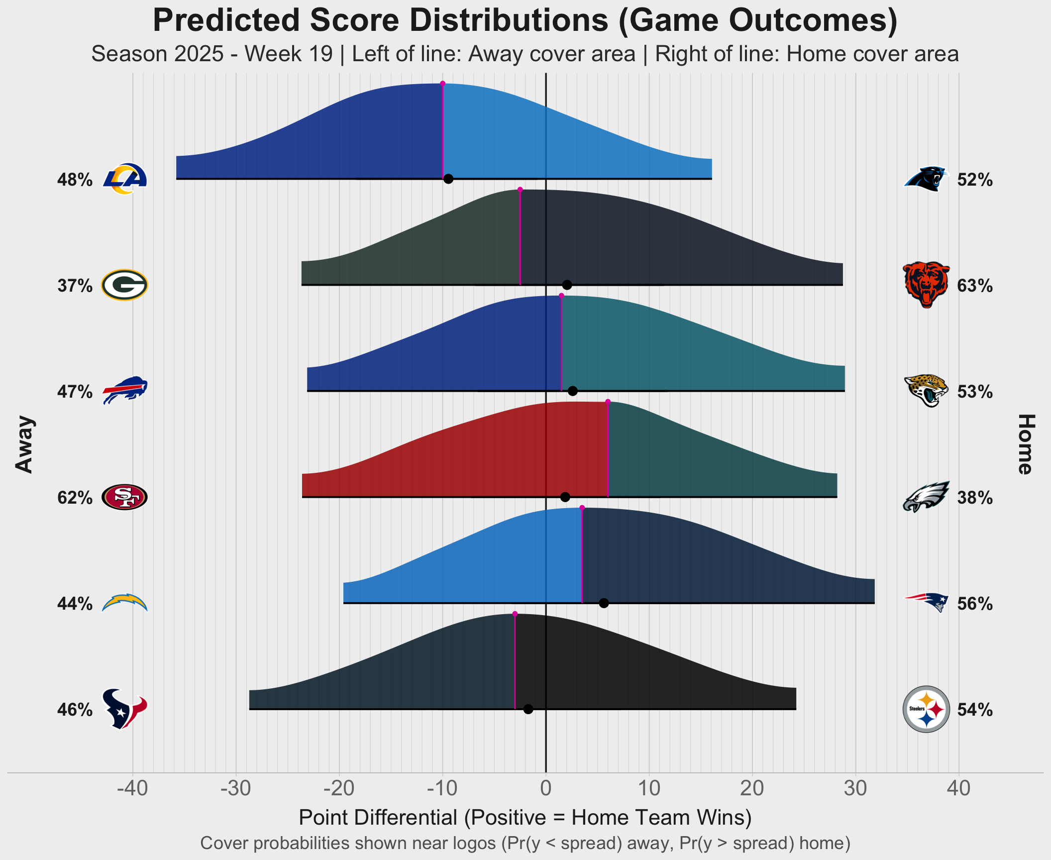
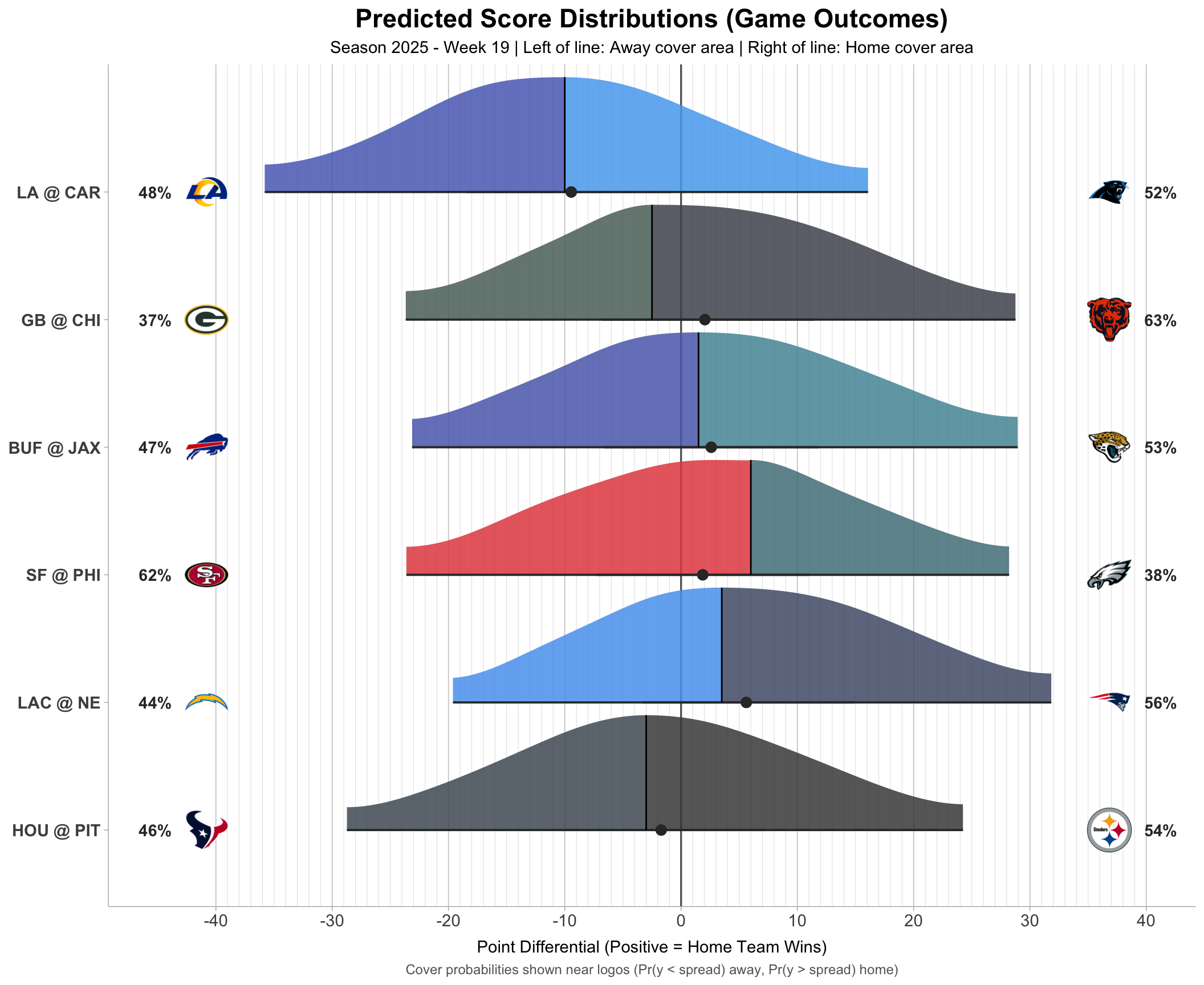
### Predicted Score Distributions
Full predictive distribution for each game showing all possible outcomes.
```{r}
#| label: score-dist-plot-new-legacy-reference
#| eval: false
#| include: false
# Old chunk retained for reference:
# ```{r}
# #| label: score-dist-plot-new
# #| code-fold: true
# #| code-summary: "Show the R code - score-dist-plot"
# #| fig-align: center
# #| fig-width: 11
# #| fig-height: 9
#
# # Calculate dynamic x-axis limits based on 95% intervals (to match trimmed slabs)
# min_y_data <- quantile(
# pred_plot_df$y,
# probs = 0.025
# ) |>
# min()
# max_y_data <- quantile(
# pred_plot_df$y,
# probs = 0.975
# ) |>
# max()
#
# # Calculate logo and text positions (relative to data bounds)
# away_logo_pos <- min_y_data - 5
# home_logo_pos <- max_y_data + 5
# away_text_pos <- min_y_data - 8
# home_text_pos <- max_y_data + 8
#
# # Calculate x-axis limits to accommodate logos/text with margin
# x_min_new <- floor((min_y_data - 8) / 5) * 5
# x_max_new <- ceiling((max_y_data + 8) / 5) * 5
#
# # Calculate 95% interval bounds for trimming (per-game)
# pred_plot_df_bounds <- pred_plot_df |>
# rowwise() |>
# mutate(
# y_lower = median(quantile(y, 0.025)),
# y_upper = median(quantile(y, 0.975))
# ) |>
# ungroup()
#
# pred_plot_df2 <- pred_plot_df_bounds |>
# tibble::as_tibble() |>
# tidybayes::unnest_rvars()
#
# # Create data subsets for two-toned slabs with smooth density
# # Filter to 95% interval to trim the tails
# pred_plot_df_away <- pred_plot_df2 |>
# filter(y >= y_lower & y <= y_upper & y < spread_line)
#
# pred_plot_df_home <- pred_plot_df2 |>
# filter(y >= y_lower & y <= y_upper & y >= spread_line)
#
# score_dist_plot_new <- pred_plot_df |>
# mutate(
# spread_line_y_prob = density(y, spread_line)
# ) |>
# ggplot(
# aes(
# y = reorder(matchup_display, game_idx, decreasing = TRUE)
# )
# ) +
# # Zero reference (home win threshold)
# geom_vline(
# xintercept = 0,
# linetype = "solid",
# color = "gray40",
# linewidth = 0.6
# ) +
# # Two-toned slab: away color below spread, home color above spread
# stat_slab(
# data = pred_plot_df_away,
# aes(
# x = y,
# y = reorder(matchup_display, game_idx, decreasing = TRUE),
# fill = away_team
# ),
# adjust = 4,
# alpha = 0.85,
# slab_linewidth = 0,
# normalize = "groups",
# show.legend = FALSE
# ) +
# stat_slab(
# data = pred_plot_df_home,
# aes(
# x = y,
# y = reorder(matchup_display, game_idx, decreasing = TRUE),
# fill = home_team
# ),
# adjust = 4,
# alpha = 0.85,
# slab_linewidth = 0,
# normalize = "groups",
# show.legend = FALSE
# ) +
# # Point interval on top
# stat_pointinterval(
# aes(xdist = y),
# point_interval = "median_qi",
# .width = c(0.5, 0.95),
# interval_color = "gray20",
# point_color = "gray20",
# point_size = 2.5,
# linewidth = 1.5
# ) +
# # Spread line marker at slab height
# stat_spike(
# aes(x = spread_line, height = spread_line_y_prob),
# size = 0
# ) +
# # Team logos (positioned relative to data bounds)
# geom_nfl_logos(
# aes(x = away_logo_pos, team_abbr = away_team),
# width = 0.045
# ) +
# geom_nfl_logos(
# aes(x = home_logo_pos, team_abbr = home_team),
# width = 0.045
# ) +
# # Cover probabilities near logos
# geom_text(
# aes(
# x = away_text_pos,
# label = scales::percent(away_y_cover_prob, accuracy = 1)
# ),
# hjust = 1,
# vjust = 0.5,
# size = 3.8,
# fontface = "bold",
# color = "gray20"
# ) +
# geom_text(
# aes(
# x = home_text_pos,
# label = scales::percent(home_y_cover_prob, accuracy = 1)
# ),
# hjust = 0,
# vjust = 0.5,
# size = 3.8,
# fontface = "bold",
# color = "gray20"
# ) +
# scale_fill_manual(
# values = colorspace::lighten(team_colors, amount = 0.30)
# ) +
# scale_x_continuous(
# breaks = seq(
# floor(min_y_data / 10) * 10,
# ceiling(max_y_data / 10) * 10,
# 10
# ),
# minor_breaks = seq(
# floor(min_y_data / 10) * 10,
# ceiling(max_y_data / 10) * 10,
# 1
# ),
# limits = c(x_min_new, x_max_new)
# ) +
# #scale_thickness_shared() +
# labs(
# title = "Predicted Score Distributions (Game Outcomes)",
# subtitle = paste(
# "Season",
# attr(predict_data$result_predict, "season"),
# "- Week",
# attr(predict_data$result_predict, "week"),
# "| Left of line: Away cover area | Right of line: Home cover area"
# ),
# x = "Point Differential (Positive = Home Team Wins)",
# y = NULL,
# caption = "Cover probabilities shown near logos (Pr(y < spread) away, Pr(y > spread) home)"
# ) +
# theme_ggdist() +
# theme(
# plot.title = element_text(size = 17, face = "bold", hjust = 0.5),
# plot.subtitle = element_text(size = 11, hjust = 0.5),
# plot.caption = element_text(size = 9, hjust = 0.5, color = "gray40"),
# axis.text.y = element_text(size = 11, face = "bold"),
# axis.text.x = element_text(size = 11),
# panel.grid.major.y = element_blank(),
# panel.grid.major.x = element_line(color = "gray80", linewidth = 0.3),
# panel.grid.minor.x = element_line(color = "gray90", linewidth = 0.2),
# legend.position = "none"
# )
#
# score_dist_plot_new
# ```
```
```{r}
#| label: score-dist-plot-new
#| renderings: [dark, light]
#| code-fold: true
#| code-summary: "Show the R code - score-dist-plot"
#| fig-align: center
#| fig-width: 11
#| fig-height: 9
# Calculate dynamic x-axis limits based on 95% intervals (to match trimmed slabs)
min_y_data <- quantile(
  pred_plot_df$y,
  probs = 0.025
) |>
  min()
max_y_data <- quantile(
  pred_plot_df$y,
  probs = 0.975
) |>
  max()

# Calculate logo and text positions (relative to data bounds)
away_logo_pos <- min_y_data - 5
home_logo_pos <- max_y_data + 5
away_text_pos <- min_y_data - 8
home_text_pos <- max_y_data + 8

# Calculate x-axis limits to accommodate logos/text with margin
x_min_new <- floor((min_y_data - 8) / 5) * 5
x_max_new <- ceiling((max_y_data + 8) / 5) * 5
away_side_label_pos <- x_min_new - 2
home_side_label_pos <- x_max_new + 2

# Calculate 95% interval bounds for trimming (per-game)
pred_plot_df_bounds <- pred_plot_df |>
  rowwise() |>
  mutate(
    y_lower = median(quantile(y, 0.025)),
    y_upper = median(quantile(y, 0.975))
  ) |>
  ungroup()

pred_plot_df2 <- pred_plot_df_bounds |>
  tibble::as_tibble() |>
  tidybayes::unnest_rvars()

# Create data subsets for two-toned slabs with smooth density
# Filter to 95% interval to trim the tails
pred_plot_df_away <- pred_plot_df2 |>
  filter(y >= y_lower & y <= y_upper & y < spread_line)

pred_plot_df_home <- pred_plot_df2 |>
  filter(y >= y_lower & y <= y_upper & y >= spread_line)

score_dist_plot_new <- pred_plot_df |>
  mutate(
    spread_line_y_prob = density(y, spread_line)
  ) |>
  ggplot(
    aes(
      y = reorder(matchup_display, game_idx, decreasing = TRUE)
    )
  ) +
  geom_vline(
    xintercept = 0,
    linetype = "solid",
    linewidth = 0.6
  ) +
  stat_slab(
    data = pred_plot_df_away,
    aes(
      x = y,
      y = reorder(matchup_display, game_idx, decreasing = TRUE),
      fill = away_team
    ),
    adjust = 4,
    alpha = 0.85,
    slab_linewidth = 0,
    normalize = "groups",
    show.legend = FALSE
  ) +
  stat_slab(
    data = pred_plot_df_home,
    aes(
      x = y,
      y = reorder(matchup_display, game_idx, decreasing = TRUE),
      fill = home_team
    ),
    adjust = 4,
    alpha = 0.85,
    slab_linewidth = 0,
    normalize = "groups",
    show.legend = FALSE
  ) +
  stat_pointinterval(
    aes(xdist = y, color = "Distribution", interval_color = "Distribution"),
    point_interval = "median_qi",
    .width = c(0.5, 0.95),
    point_size = 2.5,
    linewidth = 1.5
  ) +
  stat_spike(
    aes(
      x = spread_line,
      height = spread_line_y_prob,
      color = "Vegas"
    ),
    size = 0.9
  ) +
  geom_nfl_logos(
    aes(x = away_logo_pos, team_abbr = away_team),
    width = 0.05
  ) +
  geom_nfl_logos(
    aes(x = home_logo_pos, team_abbr = home_team),
    width = 0.05
  ) +
  annotate(
    "text",
    x = -Inf, #away_side_label_pos,
    y = (length(unique(pred_plot_df$matchup_display)) + 1) / 2,
    label = "Away",
    vjust = 1.5,
    size = base_text_size,
    size.unit = "pt",
    angle = 90,
    fontface = "bold"
  ) +
  annotate(
    "text",
    x = Inf, #home_side_label_pos,
    y = (length(unique(pred_plot_df$matchup_display)) + 1) / 2,
    label = "Home",
    vjust = 1.5,
    size = base_text_size,
    size.unit = "pt",
    angle = -90,
    fontface = "bold"
  ) +
  geom_text(
    aes(
      x = away_text_pos,
      label = scales::percent(away_y_cover_prob, accuracy = 1)
    ),
    hjust = 1,
    vjust = 0.5,
    size = base_text_size * 0.8,
    size.unit = "pt",
    fontface = "bold"
  ) +
  geom_text(
    aes(
      x = home_text_pos,
      label = scales::percent(home_y_cover_prob, accuracy = 1)
    ),
    hjust = 0,
    vjust = 0.5,
    size = base_text_size * 0.8,
    size.unit = "pt",
    fontface = "bold"
  ) +
  scale_x_continuous(
    breaks = seq(
      floor(min_y_data / 10) * 10,
      ceiling(max_y_data / 10) * 10,
      10
    ),
    minor_breaks = seq(
      floor(min_y_data / 10) * 10,
      ceiling(max_y_data / 10) * 10,
      1
    ),
    expand = expansion(mult = c(0.1, 0.1))
  ) +
  # coord_cartesian(
  #   xlim = c(x_min_new, x_max_new),
  #   clip = "off"
  # ) +
  labs(
    title = "Predicted Score Distributions (Game Outcomes)",
    subtitle = paste(
      "Season",
      attr(predict_data$result_predict, "season"),
      "- Week",
      attr(predict_data$result_predict, "week"),
      "| Left of line: Away cover area | Right of line: Home cover area"
    ),
    x = "Point Differential (Positive = Home Team Wins)",
    y = NULL,
    caption = "Cover probabilities shown near logos (Pr(y < spread) away, Pr(y > spread) home)"
  ) +
  theme_ggdist() +
  theme(
    plot.title = element_text(face = "bold", hjust = 0.5),
    plot.subtitle = element_text(size = rel(1), hjust = 0.5),
    plot.caption = element_text(size = rel(1.5), hjust = 0.5),
    axis.text.y = element_blank(),
    axis.text.x = element_text(size = rel(1.2)),
    axis.ticks.y = element_blank(),
    axis.line.y = element_blank(),
    panel.grid.major.y = element_blank(),
    panel.grid.major.x = element_line(linewidth = 0.3),
    panel.grid.minor.x = element_line(linewidth = 0.2),
    legend.position = "none"
  )

p_dark <- score_dist_plot_new
p_light <- score_dist_plot_new

p_dark +
  #scale_fill_manual(values = colorspace::lighten(team_colors, amount = 0.45)) +
  scale_fill_manual(values = team_colors) +
  scale_color_manual(
    values = c(
      Distribution = theme_brand_dark$geom$ink,
      Vegas = brand_pluck(dark_brand_yml, "color", "danger")
    )
  ) +
  scale_color_manual(
    aesthetics = "interval_colour",
    values = c(Distribution = theme_brand_dark$geom$ink)
  ) +
  theme_brand_dark

p_light +
  #scale_fill_manual(values = colorspace::lighten(team_colors, amount = 0.2)) +
  scale_fill_manual(values = team_colors) +
  scale_color_manual(
    values = c(
      Distribution = "black",
      Vegas = darken(brand_pluck(light_brand_yml, "color", "danger"), 0.2)
    )
  ) +
  scale_color_manual(
    aesthetics = "interval_colour",
    values = c(Distribution = "black")
  ) +
  theme_brand_light
```
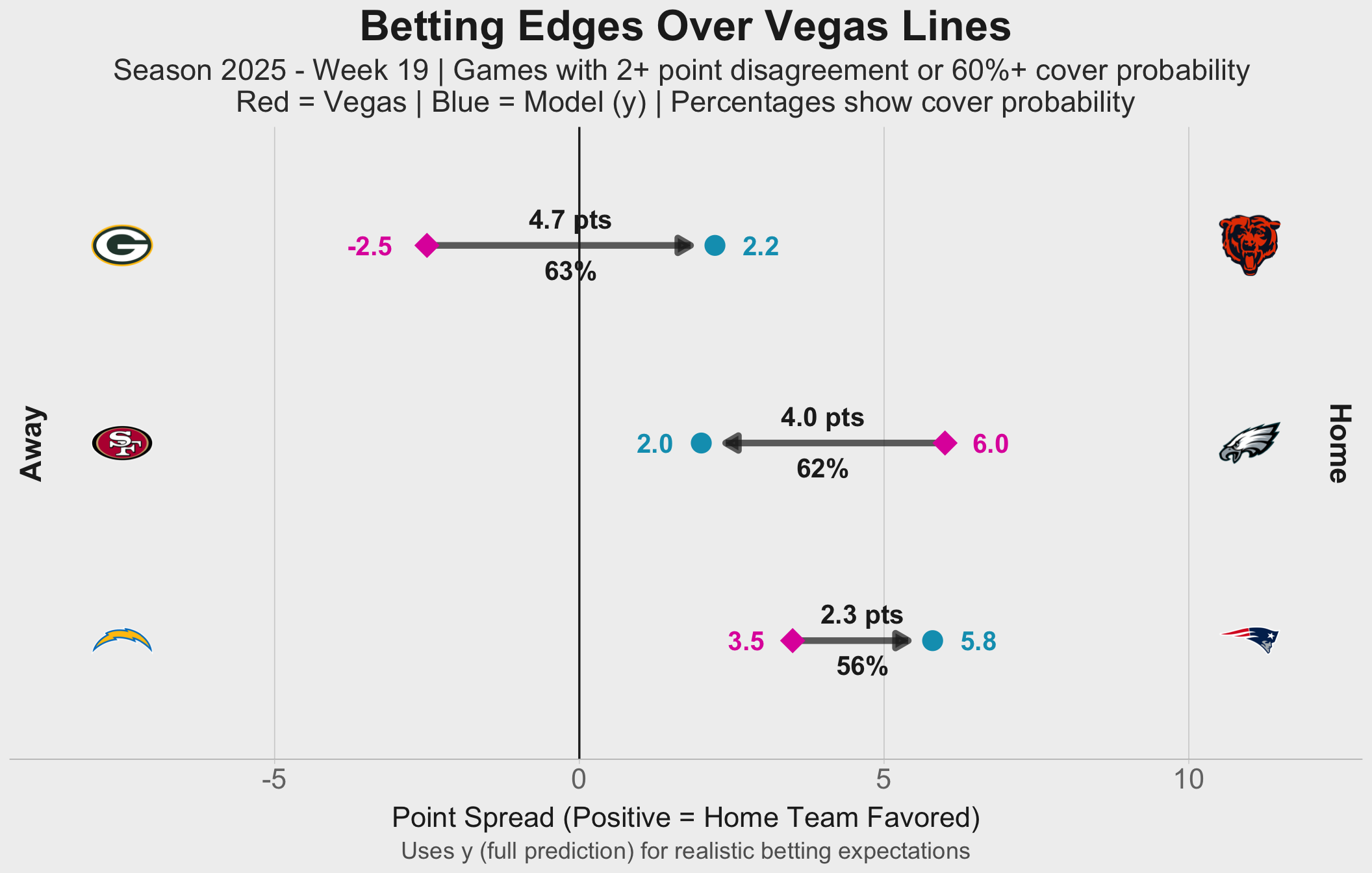
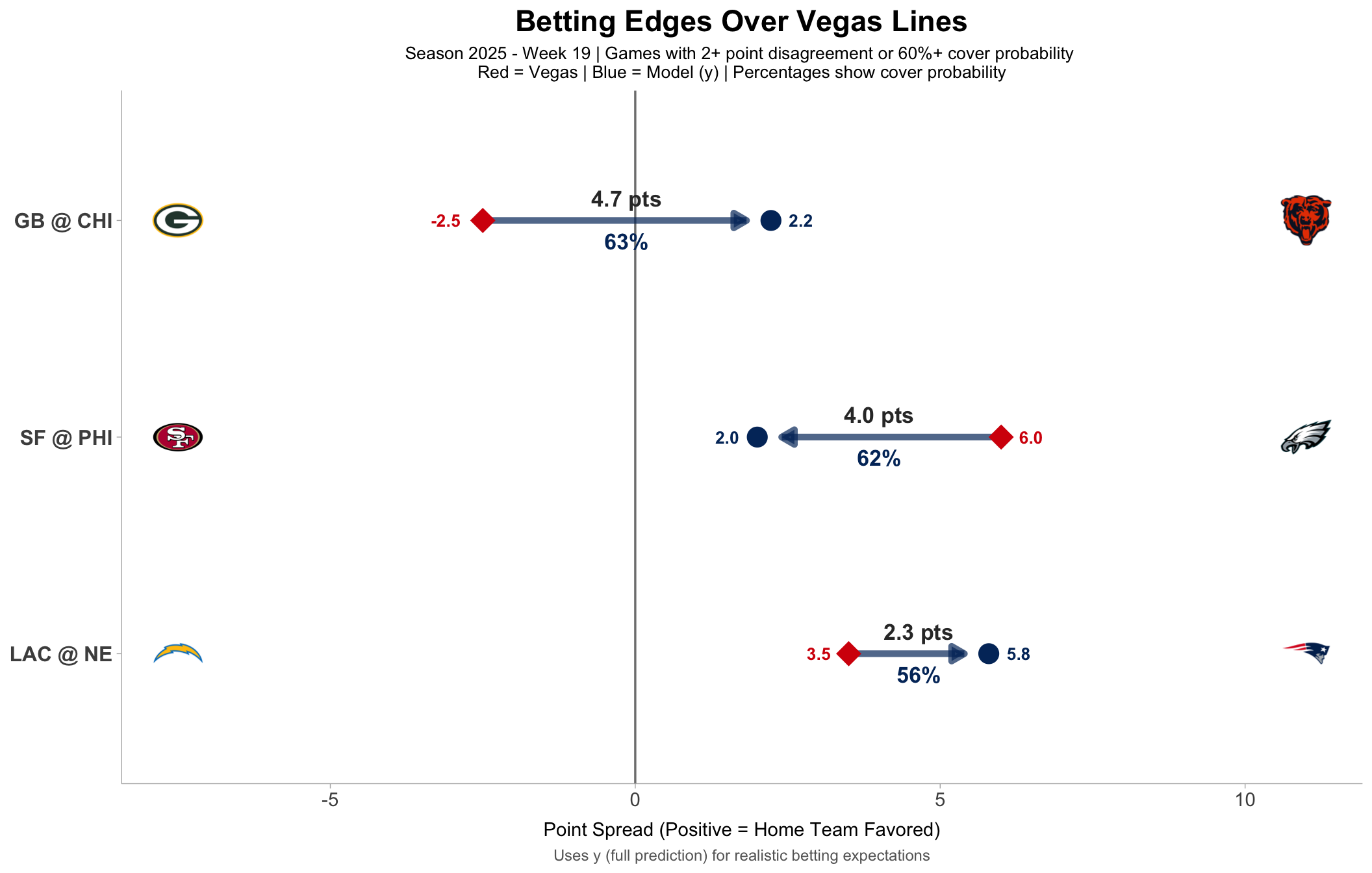
### Betting Opportunities
Games where our model disagrees with Vegas by at least 2 points or shows high confidence.
```{r}
#| label: betting-edge-plot-legacy-reference
#| eval: false
#| include: false
# Old chunk retained for reference:
# ```{r}
# #| label: betting-edge-plot
# #| code-fold: true
# #| code-summary: "Show the R code - betting-edge-plot"
# #| fig-align: center
# #| fig-width: 11
# #| fig-height: 7
#
# betting_plot <- pred_plot_df |>
# mutate(
# model_spread = E(y), # Use y for betting decisions
# spread_diff = model_spread - spread_line,
# abs_diff = abs(spread_diff),
# bet_worthy = abs_diff >= 2 | y_cover_prob >= 0.60 # Use y_cover_prob
# ) |>
# filter(bet_worthy) |>
# ggplot(aes(y = reorder(matchup_display, abs_diff))) +
# geom_vline(
# xintercept = 0,
# linetype = "solid",
# color = "gray50",
# linewidth = 0.6
# ) +
# # Arrow showing edge direction - draw first so it's under points
# # Arrow tip stops just before the point so it's visible
# geom_segment(
# aes(
# x = spread_line,
# xend = model_spread - sign(model_spread - spread_line) * 0.4,
# yend = matchup_display
# ),
# arrow = arrow(length = unit(0.3, "cm"), type = "closed"),
# linewidth = 1.8,
# color = "#013369",
# alpha = 0.7
# ) +
# # Vegas line - larger and on top
# geom_point(
# aes(x = spread_line),
# size = 6.5,
# color = "#D50A0A",
# shape = 18
# ) +
# # Model prediction - larger and on top
# geom_point(
# aes(x = model_spread),
# size = 5,
# color = "#013369"
# ) +
# # Edge label
# geom_text(
# aes(
# x = (spread_line + model_spread) / 2,
# label = sprintf("%.1f pts", abs(spread_diff))
# ),
# vjust = -0.9,
# size = 4.5,
# fontface = "bold",
# color = "gray20"
# ) +
# # Cover probability label
# geom_text(
# aes(
# x = (spread_line + model_spread) / 2,
# label = sprintf("%d%%", round(y_cover_prob * 100))
# ),
# vjust = 1.8,
# size = 4.5,
# fontface = "bold",
# color = "#013369"
# ) +
# # Spread line value label (on outside edge)
# geom_text(
# aes(
# x = spread_line,
# label = sprintf("%.1f", spread_line),
# hjust = if_else(spread_line < model_spread, 1.75, -0.75)
# ),
# vjust = 0.5,
# size = 3.5,
# fontface = "bold",
# color = "#D50A0A"
# ) +
# # Model spread value label (on outside edge)
# geom_text(
# aes(
# x = model_spread,
# label = sprintf("%.1f", model_spread),
# hjust = if_else(model_spread < spread_line, 1.75, -0.75)
# ),
# vjust = 0.5,
# size = 3.5,
# fontface = "bold",
# color = "#013369"
# ) +
# geom_nfl_logos(
# aes(x = min(c(spread_line, model_spread)) - 5, team_abbr = away_team),
# width = 0.045
# ) +
# geom_nfl_logos(
# aes(x = max(c(spread_line, model_spread)) + 5, team_abbr = home_team),
# width = 0.045
# ) +
# labs(
# title = "Betting Edges Over Vegas Lines",
# subtitle = paste(
# "Season",
# attr(predict_data$result_predict, "season"),
# "- Week",
# attr(predict_data$result_predict, "week"),
# "| Games with 2+ point disagreement or 60%+ cover probability",
# "\nRed = Vegas | Blue = Model (y) | Percentages show cover probability"
# ),
# x = "Point Spread (Positive = Home Team Favored)",
# y = NULL,
# caption = "Uses y (full prediction) for realistic betting expectations"
# ) +
# theme_ggdist() +
# theme(
# plot.title = element_text(size = 17, face = "bold", hjust = 0.5),
# plot.subtitle = element_text(size = 10, hjust = 0.5),
# plot.caption = element_text(size = 9, hjust = 0.5, color = "gray40"),
# axis.text.y = element_text(size = 12, face = "bold"),
# axis.text.x = element_text(size = 11),
# panel.grid.major.y = element_blank(),
# panel.grid.minor.x = element_blank()
# )
#
# betting_plot
# ```
```
```{r}
#| label: betting-edge-plot
#| renderings: [dark, light]
#| code-fold: true
#| code-summary: "Show the R code - betting-edge-plot"
#| fig-align: center
#| fig-width: 11
#| fig-height: 7
betting_plot_df <- pred_plot_df |>
  mutate(
    model_spread = E(y),
    spread_diff = model_spread - spread_line,
    abs_diff = abs(spread_diff),
    bet_worthy = abs_diff >= 2 | y_cover_prob >= 0.60
  ) |>
  filter(bet_worthy)

betting_min_data <- min(pmin(
  betting_plot_df$spread_line,
  betting_plot_df$model_spread
))
betting_max_data <- max(pmax(
  betting_plot_df$spread_line,
  betting_plot_df$model_spread
))
away_logo_pos_betting <- betting_min_data - 5
home_logo_pos_betting <- betting_max_data + 5
away_side_label_pos_betting <- away_logo_pos_betting - 2
home_side_label_pos_betting <- home_logo_pos_betting + 2
betting_x_min <- floor(away_logo_pos_betting / 5) * 5
betting_x_max <- ceiling(home_logo_pos_betting / 5) * 5

betting_plot <- betting_plot_df |>
  ggplot(aes(y = reorder(matchup_display, abs_diff))) +
  geom_vline(
    xintercept = 0,
    linetype = "solid",
    linewidth = 0.6
  ) +
  geom_segment(
    aes(
      x = spread_line,
      xend = model_spread - sign(model_spread - spread_line) * 0.4,
      yend = matchup_display
      #color = "Model"
    ),
    arrow = arrow(length = unit(0.3, "cm"), type = "closed"),
    linewidth = 1.8,
    alpha = 0.7
  ) +
  geom_point(
    aes(x = spread_line, color = "Vegas"),
    size = 6.5,
    shape = 18
  ) +
  geom_point(
    aes(x = model_spread, color = "Model"),
    size = 5
  ) +
  geom_text(
    aes(
      x = (spread_line + model_spread) / 2,
      label = sprintf("%.1f pts", abs(spread_diff))
      #color = "Model"
    ),
    vjust = -0.9,
    size = base_text_size * 0.9,
    size.unit = "pt",
    fontface = "bold"
  ) +
  geom_text(
    aes(
      x = (spread_line + model_spread) / 2,
      label = sprintf("%d%%", round(y_cover_prob * 100))
      #color = "Model"
    ),
    vjust = 1.8,
    size = base_text_size * 0.9,
    size.unit = "pt",
    fontface = "bold"
  ) +
  geom_text(
    aes(
      x = spread_line,
      label = sprintf("%.1f", spread_line),
      hjust = if_else(spread_line < model_spread, 1.75, -0.75),
      color = "Vegas"
    ),
    vjust = 0.5,
    size = base_text_size * 0.9,
    size.unit = "pt",
    fontface = "bold"
  ) +
  geom_text(
    aes(
      x = model_spread,
      label = sprintf("%.1f", model_spread),
      hjust = if_else(model_spread < spread_line, 1.75, -0.75),
      color = "Model"
    ),
    vjust = 0.5,
    size = base_text_size * 0.9,
    size.unit = "pt",
    fontface = "bold"
  ) +
  geom_nfl_logos(
    aes(x = away_logo_pos_betting, team_abbr = away_team),
    width = 0.05
  ) +
  geom_nfl_logos(
    aes(x = home_logo_pos_betting, team_abbr = home_team),
    width = 0.05
  ) +
  annotate(
    "text",
    x = -Inf, #away_side_label_pos_betting
    y = (length(unique(betting_plot_df$matchup_display)) + 1) / 2,
    label = "Away",
    vjust = 1.5,
    #hjust = -0.5,
    size = base_text_size,
    size.unit = "pt",
    angle = 90,
    fontface = "bold"
  ) +
  annotate(
    "text",
    x = Inf, #home_side_label_pos_betting
    y = (length(unique(betting_plot_df$matchup_display)) + 1) / 2,
    label = "Home",
    vjust = 1.5,
    #hjust = -0.5,
    size = base_text_size,
    size.unit = "pt",
    angle = -90,
    fontface = "bold"
  ) +
  scale_x_continuous(
    breaks = seq(
      floor(betting_min_data / 5) * 5,
      ceiling(betting_max_data / 5) * 5,
      5
    ),
    expand = expansion(mult = c(0.1, 0.1))
  ) +
  # coord_cartesian(
  #   xlim = c(betting_x_min, betting_x_max),
  #   clip = "off"
  # ) +
  labs(
    title = "Betting Edges Over Vegas Lines",
    subtitle = paste(
      "Season",
      attr(predict_data$result_predict, "season"),
      "- Week",
      attr(predict_data$result_predict, "week"),
      "| Games with 2+ point disagreement or 60%+ cover probability",
      "\nRed = Vegas | Blue = Model (y) | Percentages show cover probability"
    ),
    x = "Point Spread (Positive = Home Team Favored)",
    y = NULL,
    caption = "Uses y (full prediction) for realistic betting expectations"
  ) +
  theme_ggdist() +
  theme(
    plot.title = element_text(face = "bold", hjust = 0.5),
    plot.subtitle = element_text(size = rel(1), hjust = 0.5),
    plot.caption = element_text(size = rel(1.5), hjust = 0.5),
    axis.text.y = element_blank(),
    axis.text.x = element_text(size = rel(1.2)),
    axis.ticks.y = element_blank(),
    axis.line.y = element_blank(),
    panel.grid.major.y = element_blank(),
    panel.grid.major.x = element_line(linewidth = 0.3),
    panel.grid.minor.x = element_blank(),
    legend.position = "none"
  )

p_dark <- betting_plot
p_light <- betting_plot

p_dark +
  scale_color_manual(
    values = c(
      Model = brand_pluck(dark_brand_yml, "color", "info"),
      Vegas = brand_pluck(dark_brand_yml, "color", "danger")
    )
  ) +
  theme_brand_dark

p_light +
  scale_color_manual(
    values = c(
      Model = darken(brand_pluck(light_brand_yml, "color", "info"), 0.2),
      Vegas = darken(brand_pluck(light_brand_yml, "color", "danger"), 0.2)
    )
  ) +
  theme_brand_light
```